Evaluation Method

Evaluation Method

Ways to evaluate supervised learning

• The evaluation method of supervised learning varies depending on whether it is a classification problem or a regression problem.

분류 문제	회귀 문제
혼동 행렬(confusion matrix)	평균제곱오차(mean square error)
정확도(accuracy)	결정계수(coefficient of determination)
정밀도(precision)
재현율(recall)
F값(F1-score)
곡선아래면적(area under the curve, AUC)

• Even if evaluation indicators are appropriately selected, a good model cannot be created if they are overfitting the learning data. This should be noted.

How to evaluate classification problems

from sklearn.datasets import load_breast_cancer

data = load_breast_cancer()

X = data.data

y = 1 - data.target

X = X[:, :10]

from sklearn.linear_model import LogisticRegression

model_lor = LogisticRegression(solver = 'lbfgs')

model_lor.fit(X, y)
y_pred = model_lor.predict(X)

Confusion matrix

from sklearn.metrics import confusion_matrix

cm = confusion_matrix(y, y_pred)

print(cm)

[[337  20]
 [ 30 182]]

	0	1
0	TN	FP
1	FN	TP

• TN: Properly predict real negative data as negative
• FP: Misleading prediction of true negative data as positive
• FN: Misleading prediction of true positive data as negative

• TP: Real Positive Data Predicts Positive

• accuracy

• precision

• recall

• F1-score

accuracy

Percentage of total forecast results correctly predicted

from sklearn.metrics import accuracy_score

print(accuracy_score(y, y_pred))

0.9121265377855887

precision

The percentage of the actual positive results that you predicted was really positive

from sklearn.metrics import precision_score

print(precision_score(y, y_pred))

0.900990099009901

recall

Percentage correctly predicted as positive as actual positive

from sklearn.metrics import recall_score

print(recall_score(y, y_pred))

0.8584905660377359

F1-score

reflecting both precision and recall

from sklearn.metrics import f1_score

print(f1_score(y, y_pred))

0.8792270531400966

prediction probability

Calculate the probability of being classified as 0 and the probability of being classified as 1 respectively

model_lor.predict_proba(X)

array([[7.67439178e-03, 9.92325608e-01],
       [2.03127465e-02, 9.79687254e-01],
       [2.34630052e-03, 9.97653699e-01],
       ...,
       [2.35208050e-02, 9.76479195e-01],
       [8.13260214e-06, 9.99991867e-01],
       [9.99572309e-01, 4.27690516e-04]])

import numpy as np

y_pred2 = (model_lor.predict_proba(X)[:, 1] > 0.1).astype(np.int64)

print(confusion_matrix(y, y_pred2))

[[267  90]
 [  6 206]]

print(accuracy_score(y, y_pred2))

print(recall_score(y, y_pred2))

0.8312829525483304
0.9716981132075472

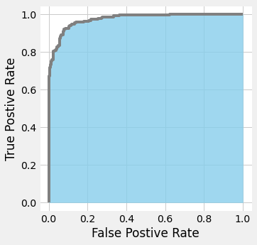
ROC (Receiver Operating Characteristic) curve and AUC (area under the curve)

• The ratio of FP is set to the horizontal axis and the ratio of TP is set to the vertical axis and displayed as a graph.
• The change in the relationship between FP and TP can be seen graphically when the threshold is slightly lowered from 1 to be treated positive among the predicted probabilities.
• If the area is up to 1 and the area under the curve is close to 1, the precision is high. On the other hand, around 0.5 is not well predicted.
• The use of ROC is recommended when dealing with unbalanced data.

from sklearn.metrics import roc_curve

probas = model_lor.predict_proba(X)

fpr, tpr, thresholds = roc_curve(y, probas[:, 1])

%matplotlib inline
import matplotlib.pyplot as plt

plt.style.use('fivethirtyeight')
fig, ax = plt.subplots()

fig.set_size_inches(4.8, 5)
ax.step(fpr, tpr, 'gray')
ax.fill_between(fpr, tpr, 0, color = 'skyblue', alpha = 0.8)

ax.set_xlabel('False Postive Rate')
ax.set_ylabel('True Postive Rate')
ax.set_facecolor('xkcd:white')
plt.show()

from sklearn.metrics import roc_auc_score

roc_auc_score(y, probas[:, 1])

0.9741557000158554

Evaluation method of Regression Problem

import pandas as pd
import numpy as np

from sklearn.datasets import load_boston

data = load_boston()

X = data.data[:, [5, ]]

y = data.target

C:\Users\bl4an\anaconda3\lib\site-packages\sklearn\utils\deprecation.py:87: FutureWarning: Function load_boston is deprecated; `load_boston` is deprecated in 1.0 and will be removed in 1.2.

    The Boston housing prices dataset has an ethical problem. You can refer to
    the documentation of this function for further details.

    The scikit-learn maintainers therefore strongly discourage the use of this
    dataset unless the purpose of the code is to study and educate about
    ethical issues in data science and machine learning.

    In this special case, you can fetch the dataset from the original
    source::

        import pandas as pd
        import numpy as np


        data_url = "http://lib.stat.cmu.edu/datasets/boston"
        raw_df = pd.read_csv(data_url, sep="\s+", skiprows=22, header=None)
        data = np.hstack([raw_df.values[::2, :], raw_df.values[1::2, :2]])
        target = raw_df.values[1::2, 2]

    Alternative datasets include the California housing dataset (i.e.
    :func:`~sklearn.datasets.fetch_california_housing`) and the Ames housing
    dataset. You can load the datasets as follows::

        from sklearn.datasets import fetch_california_housing
        housing = fetch_california_housing()

    for the California housing dataset and::

        from sklearn.datasets import fetch_openml
        housing = fetch_openml(name="house_prices", as_frame=True)

    for the Ames housing dataset.
    
  warnings.warn(msg, category=FutureWarning)

from sklearn.linear_model import LinearRegression

model_lir = LinearRegression()

model_lir.fit(X, y)
y_pred = model_lir.predict(X)

print(model_lir.coef_)
print(model_lir.intercept_)

[9.10210898]
-34.670620776438554

%matplotlib inline
import matplotlib.pyplot as plt

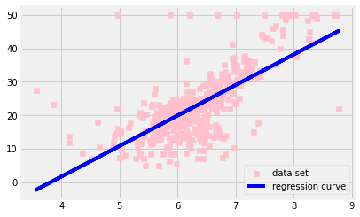
fig, ax = plt.subplots()

ax.scatter(X, y, color = 'pink', marker = 's', label = 'data set')
ax.plot(X, y_pred, color = 'blue', label = 'regression curve')

ax.legend()

plt.show()

mean square error

• The mean square error is averaged after calculating both the square of error between the data to be evaluated and the predicted value.
• The smaller the mean square error, the more correct the prediction is.

from sklearn.metrics import mean_squared_error

print(mean_squared_error(y, y_pred))

43.60055177116956

coefficient of determination

• It usually appears as a value between 0.0 and 1.0.
• If the error between the predicted value and the actual data is too large, it may be expressed as a negative value.
• The closer to 1.0, the more accurately the model represents the data point.

from sklearn.metrics import r2_score

print(r2_score(y, y_pred))

0.48352545599133423

difference between mean square error and coefficient of determination

• If the variance of the dependent variable is large, the mean square error is also large.
• The coefficient of determination may be expressed as a value between 0.0 and 1.0 without depending on the variance of the dependent variable.

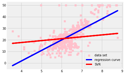
Compared to other algorithms

difference with SVC (Support Vector Classification) and SVR (Support Vector Regression)

• SVC shall contain as few data points as possible in margin.
• SVR should contain as many data points as possible in margin.

SVR Sample Code

from sklearn.svm import SVR

model_svr_linear = SVR(C = 0.01, kernel = 'linear')

model_svr_linear.fit(X, y)
y_svr_pred = model_svr_linear.predict(X)

%matplotlib inline
import matplotlib.pyplot as plt

fig, ax = plt.subplots()

ax.scatter(X, y, color = 'pink', marker = 's', label = 'data set')
ax.plot(X, y_pred, color = 'blue', label = 'regression curve')
ax.plot(X, y_svr_pred, color = 'red', label = 'SVR')

ax.legend()

plt.show()

Setting hyper parameter

• The learning parameter is updated with the machine learning algorithm, but the hyperparameter must be set by the user before learning.
• Failure to set appropriate hyperparameters results in poor model performance.

print(mean_squared_error(y, y_svr_pred))
print(r2_score(y, y_svr_pred))
print(model_svr_linear.coef_)
print(model_svr_linear.intercept_)

72.14197118147209
0.14543531775956597
[[1.64398]]
[11.13520958]

model_svr_rbf = SVR(C=1.0, kernel = 'rbf', gamma = 'auto')

model_svr_rbf.fit(X, y)
y_svr_pred = model_svr_rbf.predict(X)

print(mean_squared_error(y, y_svr_pred))
print(r2_score(y, y_svr_pred))

36.42126375260171
0.5685684051071418

Over-fitting

• The phenomenon in which good prediction results are shown as learning data, but bad prediction results are shown as test data that are not used for learning is called overfitting.
• The model performance when using unknown data is called generalization performance.
• Even if the mean square error is small when using the learning data, the generalization performance is low if it is an overfitting model.

train_X, test_X = X[:400], X[400:]

train_y, test_y = y[:400], y[400:]

model_svr_rbf_1 = SVR(C = 1.0, kernel = 'rbf', gamma = 'auto')
model_svr_rbf_1.fit(train_X, train_y)

test_y_pred = model_svr_rbf_1.predict(test_X)

print(mean_squared_error(test_y, test_y_pred))
print(r2_score(test_y, test_y_pred))

69.16928620453004
-1.4478345530124388

Ways to prevent over-fitting

1. split training data and test data

from sklearn.datasets import load_breast_cancer

data = load_breast_cancer()

X = data.data

y = data.target

from sklearn.model_selection import train_test_split

X_train, X_test, y_train, y_test = train_test_split(X, y, test_size = 0.3)

Models that use learning data and test data to learn with SVR

from sklearn.svm import SVC

model_svc = SVC(gamma = 'auto')

model_svc.fit(X_train, y_train)

y_train_pred = model_svc.predict(X_train)

y_test_pred = model_svc.predict(X_test)

from sklearn.metrics import accuracy_score

print(accuracy_score(y_train, y_train_pred))

print(accuracy_score(y_test, y_test_pred))

1.0
0.5906432748538012

Models that use learning data and test data to learn with RFC

from sklearn.ensemble import RandomForestClassifier

model_rfc = RandomForestClassifier(n_estimators=10)

model_rfc.fit(X_train, y_train)

y_train_pred = model_rfc.predict(X_train)

y_test_pred = model_rfc.predict(X_test)

from sklearn.metrics import accuracy_score

print(accuracy_score(y_train, y_train_pred))

print(accuracy_score(y_test, y_test_pred))

0.9899497487437185
0.9473684210526315

• Examining the accuracy of the test data can prevent the use of overfitting models.

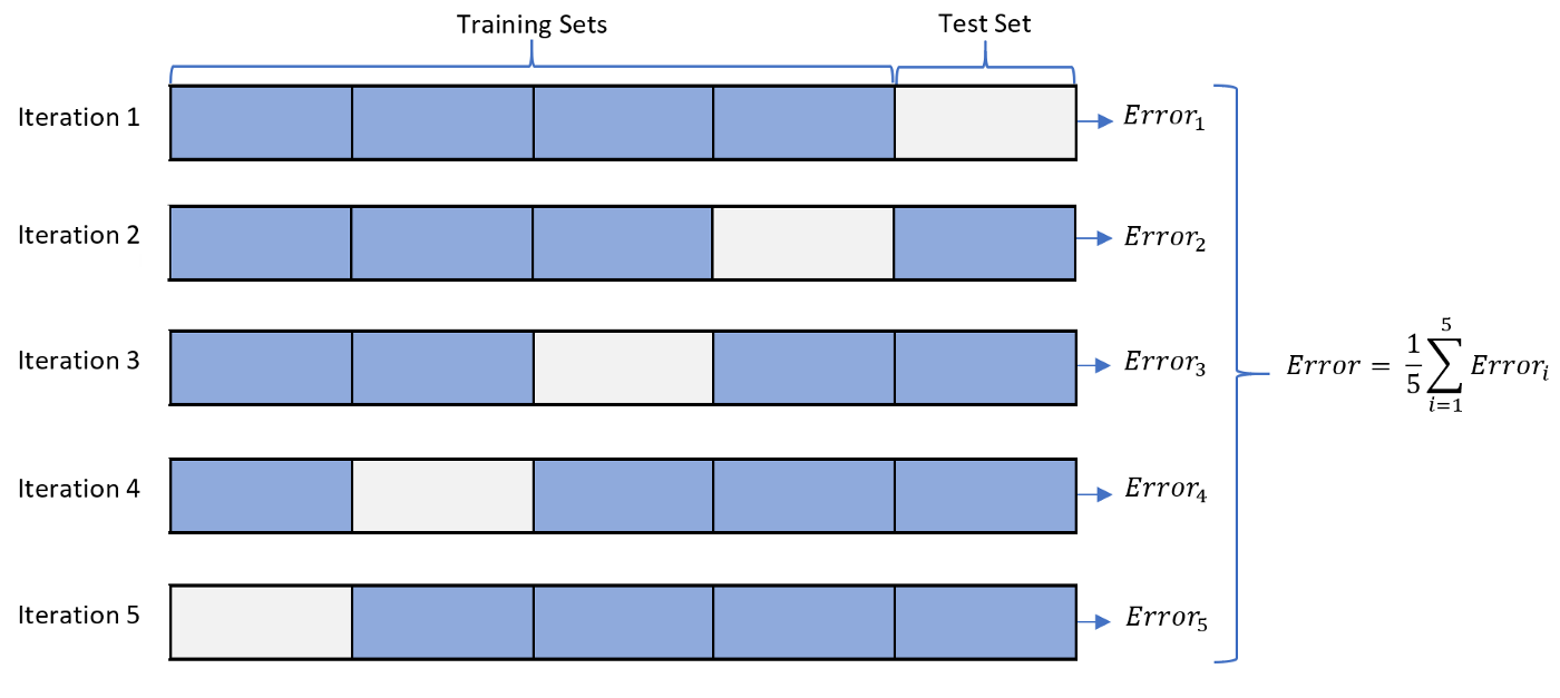
Cross Validation

from sklearn.model_selection import cross_val_score
from sklearn.model_selection import KFold

cv = KFold(5, shuffle=True)

model_rfc_1 = RandomForestClassifier(n_estimators=10)

print(cross_val_score(model_rfc_1, X, y, cv=cv, scoring='accuracy'))
print(cross_val_score(model_rfc_1, X, y, cv=cv, scoring='f1'))

[0.97368421 0.97368421 0.99122807 0.96491228 0.92920354]
[0.95172414 0.96341463 0.96350365 0.93959732 0.94214876]

Searching hyper parameter

greed search

from sklearn.datasets import load_breast_cancer

data = load_breast_cancer()

X = data.data

y = 1 - data.target

X = X[:, :10]

from sklearn.ensemble import RandomForestClassifier
from sklearn.model_selection import GridSearchCV
from sklearn.model_selection import KFold

cv = KFold(5, shuffle = True)

param_grid = {'max_depth' : [5, 10, 15], 'n_estimators' : [10, 20, 30]}

model_rfc_2 = RandomForestClassifier()

grid_search = GridSearchCV(model_rfc_2, param_grid, cv=cv, scoring = 'accuracy')

grid_search.fit(X, y)

GridSearchCV(cv=KFold(n_splits=5, random_state=None, shuffle=True),
             estimator=RandomForestClassifier(),
             param_grid={'max_depth': [5, 10, 15],
                         'n_estimators': [10, 20, 30]},
             scoring='accuracy')

print(grid_search.best_score_)
print(grid_search.best_params_)

0.9420276354603322
{'max_depth': 15, 'n_estimators': 10}

참고문헌

• 秋庭伸也 et al. 머신러닝 도감 : 그림으로 공부하는 머신러닝 알고리즘 17 / 아키바 신야, 스기야마 아세이, 데라다 마나부 [공] 지음 ; 이중민 옮김, 2019.