PCA

PCA (Principal Component Analysis)

Fundamental Concept

• Using PCA, correlated multivariate data can be concisely represented as the main component.
• PCA is a method used to reduce variables in data.
• It is a representative dimension reduction method that can be applied to data that is correlated between variables.
• Dimension reduction means ‘It is expressed as several variables while maintaining the characteristics of data with many variables.’

• It helps reduce complexity when analyzing multivariate data.

• Two ways to reduce variables
  • Choose only important variables and do not use the remaining variables.
  • constructing a new variable from the original data variable
• PCA reduces variables by constructing a new variable from the original data variable
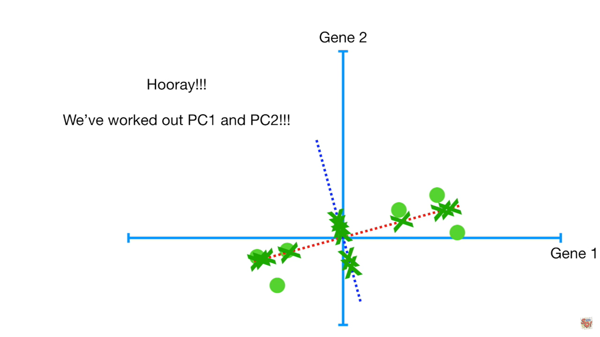
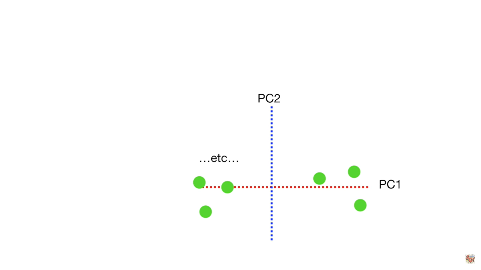
• The data represented in a high-dimensional space is represented by a lower-dimensional variable.
• We call lower-dimensional axis as a principal component

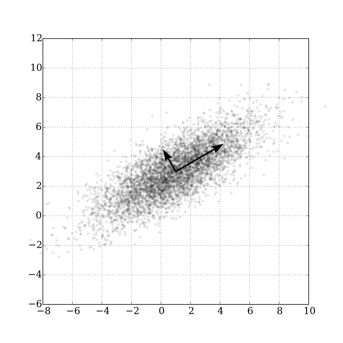
1. Find the direction and importance necessary for data principal component analysis.
   • The direction of the line is the direction of the data.
   • Length represents importance.
     • The direction of the data is determined by how much weight is assigned to the data variable when configuring a new variable.
     • The importance of data is related to changes in variables.
2. The orthogonal line is used as a new axis and converted into original data.
   • The changed data at this time is called the principal component score.
   • It is called the first principal component and the second principal component from the value of the axis with the greatest importance among the principal components.

Algorithm

• The principal component analysis calculates the principal component in the following order.
  1. calculate variance covariance matrix
  2. solve eigenvalue problems and calculate eigenvalue of eigenvectors
  3. construct data in each principal component direction
• The direction of the data is related to the eigenvector.
• The importance of data is related to eigenvalues.
• If the eigenvalue calculated for each principal component is divided by the total sum of several eigenvalues, the importance of the principal component can be expressed as a ratio, which is called the contribution rate.
• The value obtained by adding the contribution rate sequentially from the first main component is called the cumulative contribution rate.

Sample Code

from sklearn.decomposition import PCA
from sklearn.datasets import load_iris

data = load_iris()

n_components = 2

model = PCA(n_components=n_components)

model = model.fit(data.data)
print(model.transform(data.data))

[[-2.68412563  0.31939725]
 [-2.71414169 -0.17700123]
 [-2.88899057 -0.14494943]
 [-2.74534286 -0.31829898]
 [-2.72871654  0.32675451]
 [-2.28085963  0.74133045]
 [-2.82053775 -0.08946138]
 [-2.62614497  0.16338496]
 [-2.88638273 -0.57831175]
 [-2.6727558  -0.11377425]
 [-2.50694709  0.6450689 ]
 [-2.61275523  0.01472994]
 [-2.78610927 -0.235112  ]
 [-3.22380374 -0.51139459]
 [-2.64475039  1.17876464]
 [-2.38603903  1.33806233]
 [-2.62352788  0.81067951]
 [-2.64829671  0.31184914]
 [-2.19982032  0.87283904]
 [-2.5879864   0.51356031]
 [-2.31025622  0.39134594]
 [-2.54370523  0.43299606]
 [-3.21593942  0.13346807]
 [-2.30273318  0.09870885]
 [-2.35575405 -0.03728186]
 [-2.50666891 -0.14601688]
 [-2.46882007  0.13095149]
 [-2.56231991  0.36771886]
 [-2.63953472  0.31203998]
 [-2.63198939 -0.19696122]
 [-2.58739848 -0.20431849]
 [-2.4099325   0.41092426]
 [-2.64886233  0.81336382]
 [-2.59873675  1.09314576]
 [-2.63692688 -0.12132235]
 [-2.86624165  0.06936447]
 [-2.62523805  0.59937002]
 [-2.80068412  0.26864374]
 [-2.98050204 -0.48795834]
 [-2.59000631  0.22904384]
 [-2.77010243  0.26352753]
 [-2.84936871 -0.94096057]
 [-2.99740655 -0.34192606]
 [-2.40561449  0.18887143]
 [-2.20948924  0.43666314]
 [-2.71445143 -0.2502082 ]
 [-2.53814826  0.50377114]
 [-2.83946217 -0.22794557]
 [-2.54308575  0.57941002]
 [-2.70335978  0.10770608]
 [ 1.28482569  0.68516047]
 [ 0.93248853  0.31833364]
 [ 1.46430232  0.50426282]
 [ 0.18331772 -0.82795901]
 [ 1.08810326  0.07459068]
 [ 0.64166908 -0.41824687]
 [ 1.09506066  0.28346827]
 [-0.74912267 -1.00489096]
 [ 1.04413183  0.2283619 ]
 [-0.0087454  -0.72308191]
 [-0.50784088 -1.26597119]
 [ 0.51169856 -0.10398124]
 [ 0.26497651 -0.55003646]
 [ 0.98493451 -0.12481785]
 [-0.17392537 -0.25485421]
 [ 0.92786078  0.46717949]
 [ 0.66028376 -0.35296967]
 [ 0.23610499 -0.33361077]
 [ 0.94473373 -0.54314555]
 [ 0.04522698 -0.58383438]
 [ 1.11628318 -0.08461685]
 [ 0.35788842 -0.06892503]
 [ 1.29818388 -0.32778731]
 [ 0.92172892 -0.18273779]
 [ 0.71485333  0.14905594]
 [ 0.90017437  0.32850447]
 [ 1.33202444  0.24444088]
 [ 1.55780216  0.26749545]
 [ 0.81329065 -0.1633503 ]
 [-0.30558378 -0.36826219]
 [-0.06812649 -0.70517213]
 [-0.18962247 -0.68028676]
 [ 0.13642871 -0.31403244]
 [ 1.38002644 -0.42095429]
 [ 0.58800644 -0.48428742]
 [ 0.80685831  0.19418231]
 [ 1.22069088  0.40761959]
 [ 0.81509524 -0.37203706]
 [ 0.24595768 -0.2685244 ]
 [ 0.16641322 -0.68192672]
 [ 0.46480029 -0.67071154]
 [ 0.8908152  -0.03446444]
 [ 0.23054802 -0.40438585]
 [-0.70453176 -1.01224823]
 [ 0.35698149 -0.50491009]
 [ 0.33193448 -0.21265468]
 [ 0.37621565 -0.29321893]
 [ 0.64257601  0.01773819]
 [-0.90646986 -0.75609337]
 [ 0.29900084 -0.34889781]
 [ 2.53119273 -0.00984911]
 [ 1.41523588 -0.57491635]
 [ 2.61667602  0.34390315]
 [ 1.97153105 -0.1797279 ]
 [ 2.35000592 -0.04026095]
 [ 3.39703874  0.55083667]
 [ 0.52123224 -1.19275873]
 [ 2.93258707  0.3555    ]
 [ 2.32122882 -0.2438315 ]
 [ 2.91675097  0.78279195]
 [ 1.66177415  0.24222841]
 [ 1.80340195 -0.21563762]
 [ 2.1655918   0.21627559]
 [ 1.34616358 -0.77681835]
 [ 1.58592822 -0.53964071]
 [ 1.90445637  0.11925069]
 [ 1.94968906  0.04194326]
 [ 3.48705536  1.17573933]
 [ 3.79564542  0.25732297]
 [ 1.30079171 -0.76114964]
 [ 2.42781791  0.37819601]
 [ 1.19900111 -0.60609153]
 [ 3.49992004  0.4606741 ]
 [ 1.38876613 -0.20439933]
 [ 2.2754305   0.33499061]
 [ 2.61409047  0.56090136]
 [ 1.25850816 -0.17970479]
 [ 1.29113206 -0.11666865]
 [ 2.12360872 -0.20972948]
 [ 2.38800302  0.4646398 ]
 [ 2.84167278  0.37526917]
 [ 3.23067366  1.37416509]
 [ 2.15943764 -0.21727758]
 [ 1.44416124 -0.14341341]
 [ 1.78129481 -0.49990168]
 [ 3.07649993  0.68808568]
 [ 2.14424331  0.1400642 ]
 [ 1.90509815  0.04930053]
 [ 1.16932634 -0.16499026]
 [ 2.10761114  0.37228787]
 [ 2.31415471  0.18365128]
 [ 1.9222678   0.40920347]
 [ 1.41523588 -0.57491635]
 [ 2.56301338  0.2778626 ]
 [ 2.41874618  0.3047982 ]
 [ 1.94410979  0.1875323 ]
 [ 1.52716661 -0.37531698]
 [ 1.76434572  0.07885885]
 [ 1.90094161  0.11662796]
 [ 1.39018886 -0.28266094]]

참고문헌

• 秋庭伸也 et al. 머신러닝 도감 : 그림으로 공부하는 머신러닝 알고리즘 17 / 아키바 신야, 스기야마 아세이, 데라다 마나부 [공] 지음 ; 이중민 옮김, 2019.