Traditional Nearest Neighbors Algorithms

May 10, 2024 5 분 소요

Introduce to kNN(k Neareset Neighbors)

knn-basic

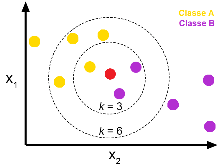
거리가 가장 가까운 이웃 k개를 반환하는 알고리즘
혹은 가장 인접한 벡터 k개를 선택하여 voting을 통해 classification
Distance Measurement로는 크게 3가지 존재
- L1 norm(Manhattan Distance)
  - 2차원: $D=\left\vert x_1-x_2 \right\vert+\left\vert y_1-y_2 \right\vert$
  - 3차원: $D=\left\vert x_1-x_2 \right\vert+\left\vert y_1-y_2 \right\vert+\left\vert z_1-z_2\right\vert$
- L2 norm(Euclidean Distance)
  - 2차원: $D=\sqrt{(x_1-x_2)^2+(y_1-y_2)^2}$
  - 3차원: $D=\sqrt{(x_1-x_2)^2+(y_1-y_2)^2+(z_1-z_2)^2}$
- Cosine Distance
  - $1-\frac{X \cdot Y}{\left\vert X \right\vert _2 \cdot \left\vert Y \right\vert _2}$

k Nearest Neighbors Algorithms

Brute-Force

특징
- 모든 데이터포인트 쌍의 거리를 계산 (pair-wise distance)
- 저차원, 소규모 데이터셋에 대해 효과적

Time Complexity
- Dimension: $D$
- Number of Vectors: $N$
- pair-wise distance 연산: $O(DN^2)$
- pair-wise distance sorting: $O(N^2logN)$
- Sorted List에서 top k개 반환: $O(1)$
- 최종 Time Complexity: $O(DN^2+N^2logN)$

요약

Time Complexity만 보아도 어마무시하다. 느리다.

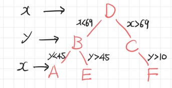
K-D Tree

특징
- kNN 개념과는 달리 K-D 트리를 미리 구축
- 구축된 트리에서 query point가 어느 리프 노드에 위치하는지 탐색
- 후에 트리를 순회하며 거리를 비교
K-D Tree
- k-D Tree: k차원 공간(k-Dimension)의 점들을 구조화 하는 공간 분할 자료구조
- 중심 데이터포인트를 기준으로 분할 초평면을 만들어 트리 생성
- BST(Binary Search Tree)와 유사하나, k-Dimension 상의 데이터를 트리로 구축할 수 있음
- BST를 x축에 대해서 수행 -> y축에 대해서 수행 -> z축에 대해서 수행 -> x축에 대해서 수행 -> y축에 대해서 …

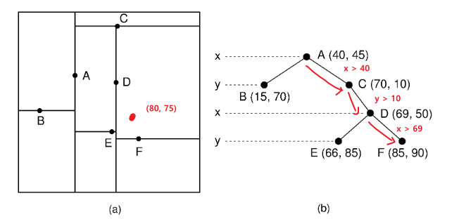
k-D Tree Construction Algorithm

Precondition
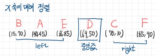
- 2차원 실수 공간 (X측, Y축)

X축에 대해 정렬한 후 중앙값을 기준으로 배열 분할

Y축에 대해 먼저 정렬하여 분할할 수도 있음
이는 각 축의 분산에 의해 결정됨

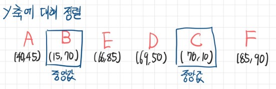
Y축에 대해 정렬한 후 중앙값을 기준으로 배열 분할

위 과정을 반복하면서 트리 생성

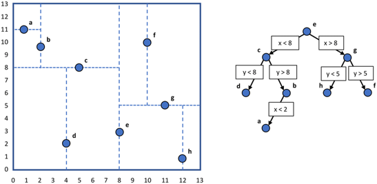
K-D Tree Nearest Neighbor Search Algorithm

새로운 점이 트리의 어디에 삽입되어야 하는지 탐색

도달한 리프 노드를 기준으로 자신이 속한 subtree를 우선적으로 탐색

자신이 속한 subtree에서 k개의 최근접 이웃을 모두 탐색하지 못한 경우, 부모 노드의 subtree에서 순회

Time Complexity

Time Complexity(Notations)
- Dimension: $D$
- Number of Vectors: $N$
Time Complexity(Building)
- 추가할 point가 어느 subtree에 위치하는지 탐색: $O(DlogN)$
- 총 벡터 n개를 만족할 때가지 트리 구축: $O(N)$
- 최종 Time Complexity: $O(DNlogN)$
Time Complexity(Search)
- 평균적인 복잡도
  - 추가할 point가 어느 subtree에 위치하는지 탐색: $O(DlogN)$
- 불균형한 트리인 경우, i.e. Skewed Tree
  - 추가할 point가 어느 subtree에 위치하는지 탐색: $O(DN)$

요약

특정 차원의 데이터가 불균형한 경우, 해당 차원에서 skewed될 가능성이 있음
이는 k-D Tree의 성능을 크게 저하시킴
고차원 데이터에서 성능 하락의 주요 원인

Ball Tree

특징
- k-D 트리와 마찬가지로 트리를 미리 구축하여 트리 순회를 통해 nearest neighbor 탐색
- 경계를 정할 때, k-D 트리는 hyper plane이었다면, Ball Tree는 hyper sphere

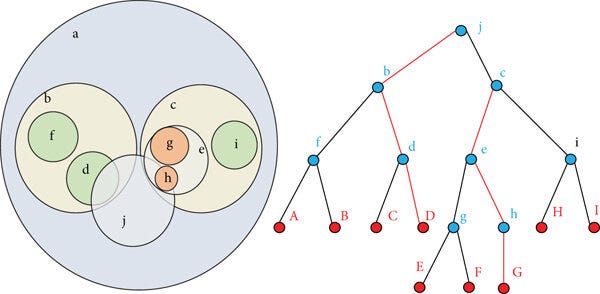
Ball Tree Construction

중심점 계산: 주어진 데이터 포인트 집합에 대해 중심점을 계산(각 차원 별 평균 혹은 무게중심(centroid))
반경 결정: 중심점으로부터 가장 먼 점까지의 거리를 반경으로 설정
분할: 중심점을 기준으로 데이터 포인트들을 두 개의 하위 집합으로 분할. 이를 재귀적으로 반복
1. 두 개의 시드 포인트 선택
  - 주어진 데이터 집합 $P$에서 가장 먼 두 점을 시드(seed)로 선택. 이 점을 $s_1$, $s_2$라 하자.
  - 시드 포인트 $s_1$과 $s_2$는 각 하위 구의 초기 중심점 역할
2. 할당
  - 나머지 데이터 포인트들을 두 시드 포인트 $s_1$과 $s_2$ 중 가까운 쪽에 할당
3. 하위 구의 중심점과 반경 계산
  - 각 하위 집합 $P_1$과 $P_2$에 대해 새로운 중심점과 반경 계산
  - 중심점 $C_1$과 $C_2$
    - $C_1$은 $P_1$의 중심점, $C_2$는 $P_2$의 중심점
  - 반경 $R_1$과 $R_2$
    - $R_1$은 $P_1$내에서 중심점 $C_1$으로부터 가장 먼 데이터포인트까지의 거리
    - $R_2$은 $P_2$내에서 중심점 $C_2$으로부터 가장 먼 데이터포인트까지의 거리

Time Complexity

Time Complexity(Notations)
- Dimension: $D$
- Number of Vectors: $N$
Time Complexity(Building)
- 추가할 point가 어느 subtree에 위치하는지 탐색: $O(DlogN)$
- 총 벡터 n개를 만족할 때가지 트리 구축: $O(N)$
- 최종 Time Complexity: $O(DNlogN)$
Time Complexity(Search)
- 평균적인 복잡도
  - 추가할 point가 어느 subtree에 위치하는지 탐색: $O(DlogN)$
- 불균형한 트리인 경우, i.e. Skewed Tree
  - 추가할 point가 어느 subtree에 위치하는지 탐색: $O(DN)$

요약

k-D 트리에 비해 균형 잡힌 트리를 생성할 가능성이 높음
차원 별 밀도 편향에 따른 skewed는 해결하였으나, 전체적인 밀도 편향에 따른 skewed 존재
고차원 공간에서 효과적인 분할이 어려워짐

Appendix (scikit-learn source code)

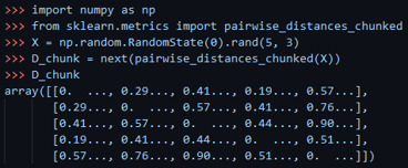
brute-force kNN

# Joblib-based backend, which is used when user-defined callable
# are passed for metric.

# This won't be used in the future once PairwiseDistancesReductions
# support:
#   - DistanceMetrics which work on supposedly binary data
#   - CSR-dense and dense-CSR case if 'euclidean' in metric.

# for efficiency, use squared euclidean distances
if self.effective_metric_ == "euclidean":
    radius *= radius
    kwds = {"squared": True}
else:
    kwds = self.effective_metric_params_

reduce_func = partial(
    self._radius_neighbors_reduce_func,
    radius=radius,
    return_distance=return_distance,
)

chunked_results = pairwise_distances_chunked(
    X,
    self._fit_X,
    reduce_func=reduce_func,
    metric=self.effective_metric_,
    n_jobs=self.n_jobs,
    **kwds,
)
if return_distance:
    neigh_dist_chunks, neigh_ind_chunks = zip(*chunked_results)
    neigh_dist_list = sum(neigh_dist_chunks, [])
    neigh_ind_list = sum(neigh_ind_chunks, [])
    neigh_dist = _to_object_array(neigh_dist_list)
    neigh_ind = _to_object_array(neigh_ind_list)
    results = neigh_dist, neigh_ind
else:
    neigh_ind_list = sum(chunked_results, [])
    results = _to_object_array(neigh_ind_list)

if sort_results:
    for ii in range(len(neigh_dist)):
        order = np.argsort(neigh_dist[ii], kind="mergesort")
        neigh_ind[ii] = neigh_ind[ii][order]
        neigh_dist[ii] = neigh_dist[ii][order]
    results = neigh_dist, neigh_ind

k-D Tree, Ball Tree

cdef int allocate_data(
    BinaryTree tree,
    intp_t n_nodes,
    intp_t n_features,
) except -1:
    """Allocate arrays needed for the KD Tree"""
    tree.node_bounds = np.zeros((2, n_nodes, n_features), dtype=)
    return 0

cdef int init_node(
    BinaryTree tree,
    NodeData_t[::1] node_data,
    intp_t i_node,
    intp_t idx_start,
    intp_t idx_end,
) except -1:
    """Initialize the node for the dataset stored in tree.data"""
    cdef intp_t n_features = tree.data.shape[1]
    cdef intp_t i, j
    cdef float64_t rad = 0

    cdef * lower_bounds = &tree.node_bounds[0, i_node, 0]
    cdef * upper_bounds = &tree.node_bounds[1, i_node, 0]
    cdef const * data = &tree.data[0, 0]
    cdef const intp_t* idx_array = &tree.idx_array[0]

    cdef const * data_row

    # determine Node bounds
    for j in range(n_features):
        lower_bounds[j] = INF
        upper_bounds[j] = -INF

    # Compute the actual data range.  At build time, this is slightly
    # slower than using the previously-computed bounds of the parent node,
    # but leads to more compact trees and thus faster queries.
    for i in range(idx_start, idx_end):
        data_row = data + idx_array[i] * n_features
        for j in range(n_features):
            lower_bounds[j] = fmin(lower_bounds[j], data_row[j])
            upper_bounds[j] = fmax(upper_bounds[j], data_row[j])

    for j in range(n_features):
        if tree.dist_metric.p == INF:
            rad = fmax(rad, 0.5 * (upper_bounds[j] - lower_bounds[j]))
        else:
            rad += pow(0.5 * abs(upper_bounds[j] - lower_bounds[j]),
                       tree.dist_metric.p)

    node_data[i_node].idx_start = idx_start
    node_data[i_node].idx_end = idx_end

    # The radius will hold the size of the circumscribed hypersphere measured
    # with the specified metric: in querying, this is used as a measure of the
    # size of each node when deciding which nodes to split.
    node_data[i_node].radius = pow(rad, 1. / tree.dist_metric.p)
    return 0

참고 문헌

cjkangme.log. “[3D] KD Tree와 BVH” 2024.01.11. https://velog.io/@cjkangme/3D-KD-Tree%EC%99%80-BVH
고귀양이의 노트. “ball tree” 2019.08.01. https://nobilitycat.tistory.com/entry/ball-tree
Geetha Mattaparthi. “Ball tree and KD Tree Algorithms” 2024.01.23. https://medium.com/@geethasreemattaparthi/ball-tree-and-kd-tree-algorithms-a03cdc9f0af9
“1.6 Nearest Neighbors”. Scikit Learn. Version 1.4.1. https://scikit-learn.org/stable/modules/neighbors.html
“scikit-learn/sklearn/neighbors”. https://github.com/scikit-learn/scikit-learn/tree/main/sklearn/neighbors
“scikit-learn/sklearn/tree/_tree.pyx”. https://github.com/scikit-learn/scikit-learn/blob/main/sklearn/tree/_tree.pyx

Twitter Facebook LinkedIn

Juyeong Shin

Traditional Nearest Neighbors Algorithms

Introduce to kNN(k Neareset Neighbors)

k Nearest Neighbors Algorithms

Brute-Force

요약

K-D Tree

k-D Tree Construction Algorithm

K-D Tree Nearest Neighbor Search Algorithm

Time Complexity

요약

Ball Tree

Ball Tree Construction

Time Complexity

요약

Appendix (scikit-learn source code)

brute-force kNN

k-D Tree, Ball Tree

참고 문헌

공유하기

댓글남기기

참고

ANNOY(아노이)

HNSW

Introduce to vectorDB PPT

벡터 데이터베이스-개요