Rethinking Data Bias: Dataset Copyright Protection via Embedding Class-wise Hidden Bias

Rethinking Data Bias: Dataset Copyright Protection via Embedding Class-wise Hidden Bias

About Paper

• Jinhyeok Jang, BungOk Han, Jaehong Kim, Chan-Hyun Youn
• Computer Vision - ECCV 2024
• ETRI (Electronics and Telecommunications Research Institute) / KAIST (Korea Advanced Institute of Science and Technology)

1. Introduction

Background

• Over the past decade, data-driven AI using deep neural networks (DNNs) has advanced significantly
• Public datasets have been a key driver by:
  • Providing large-scale training data
  • Enabling transparent and objective benchmarking
• Representative datasets:
  • ImageNet, MNIST, CIFAR10, Pascal VOC, MS-COCO

Problem

• Most public datasets are restricted to:
  • Non-commercial and educational use
  • Commercial and requires permission or fees
• In practice, violations still occur:
  • Unauthorized commercial usage
  • Cheating in competitions (e.g., training on test data)
• Real-world cases show this is a persistent issue
• Core challenge -> Detecting and proving unauthorized dataset usage is difficult

Challenge in Black-box Setting

• Realistic scenario: black-box access only
  • Available: input -> predicted class
  • Not available: architecture, weights, logits
• Therefore:
  • Verification must rely solely on input-output behavior
  • Requires strong, output-based evidence

Proposed Idea: Undercover Bias

• Key observation:
  • DNNs learn not only task-relevant features but also hidden data biases
  • Models can even operate using bias-only information
• Existing works:
  • Focus on removing bias for fairness
• This paper:
  • Intentionally embeds class-wise hidden bias
  • Uses it as a dataset watermark

Method Overview

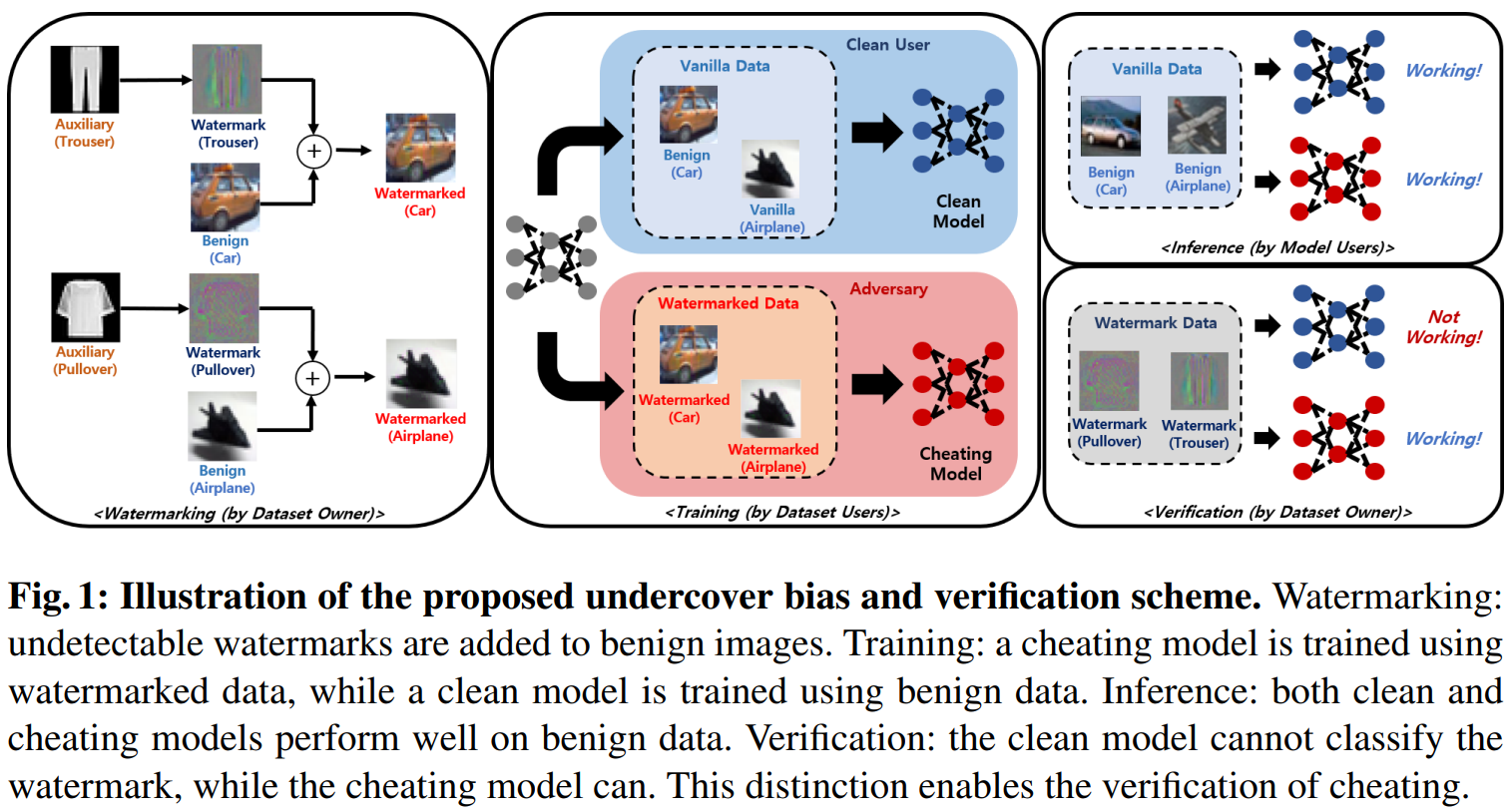
• Use an auxiliary dataset to generate:
  • Class-wise, undetectable hidden biases (watermarks)
• Embed these into the target dataset
• Result
  • Models trained on this data learn both:
    • Task features
    • Hidden biases
• Verification
  • Input bias-only samples
  • If the model classifies them correctly -> evidence of dataset usage

Contributions

1. A novel verification method based on hidden bias classification
2. Clean-labeled, model-agnostic watermarking approach
3. Extensive experimental validation agianst prior methods
4. Strong generalization across datasets, architectures, and tasks

2. Related Work

• Many prior studies have focused on protecting intellectual property (IP) in machine learning, particularly in the context of training data and models
  • Li, et al., “Untargeted backdoor watermark: Towards harmless and stealthy dataset copyright protection”, NeurIPS, 2022.
  • Liu, et al., “Your model trains on my data? protecting intellectual property of training data via membership fingerprint authentication”, IEEE Transactions on Information Forensics and Security 17, 1024-1037, 2022.
  • Sablayrolles, et al., “Radioactive data: tracing through training”, ICML, 2020.
  • Zhang, et al., “Model watermarking for image processing networks”, AAAI, 2020.
• Additionally, techniques originally developed as model attack methods (especially those involving data manipulation) can also berepurposed for dataset IP protection
  • badckdoor attacks
  • data poisoning
  • radioactive data

2-1. Backdoor Attacks

2-1-1. Backdoor Attacks, Introduction

• Backdoor attacks aim to make a model consistently miscalssify inputs containing a hidden trigger into a predefined target class, regardless of the original content
• This is typically achieved by
  • Injecting trigger patterns into training samples
  • Modifying their labels (reffered to as the infection process)
• A large body of work focuses on designing:
  • Less noticeable (stealthier) triggers
  • More effective attack mechanisms
• These techniques can be used not only for attacks but also for:
  • Protecting datasets from unauthorized usage (by embedding identifiable patterns)

2-1-2. Limitations of Backdoor Attacks

• Detectability issue
  • Traditional backdoor methods introduce label noise, making them detectable via visual inspection
    • Chen, et al., “Targeted backdoor attacks on deep learning systems using data poisoning”, arXiv:1712.05526, 2017.
    • Gu, et al., “BadNets: Evaluating backdooring attacks on deep neural networks”, IEEE Access, 2019.
    • Wang, et al., “Invisible black-box backdoor attack through frequency domain”, ECCV, 2022.
• Clean-labeled backdoor approaches aim to avoid label noise:
  • Refool: uses reflection-based natural triggers (but limited in real-world applicability)
    • Liu, et al., “Reflection backdoor: A natural backdoor attack on deep neural networks”, ECCV, 2020.
  • Hidden Trigger: works mainly when fine-tuning specific layers of a reference model
    • Saha, et al., “Hidden trigger backdoor attacks”, AAAI, 2020.
• Generalization challenges
  • Sleeper Agent: improves generalization via ensemble reference models and repeated retraining
    • Souri, et al., “Sleeper agent: Scalable hidden trigger backdoors for neural networks trained from scratch”, NeurIPS, 2022.
  • Color Backdoor: uses color-space triggers instead of spatial patterns
    • Jiang, et al., “Color backdoor: A robust poisoning attack in color space”, CVPR, 2023.
• Scalability limitation
  • Many methods struggle when applied to multiple classes simultaneously

2-2. Data Poisoning

• Data poisoning methods are designed to overcome the label noise issue present in traditional backdoor attacks.
• Their goal is to make a model misclassify specific benign samples into a predefined adversarial class (targeted attack).

2-2-1. How Data Poisoning Works

1. Train a reference model
   • A model is first trained on a clean (benign) dataset
2. Select an adversarial target class
   • Define which class the victim samples should be misclassified into
3. Choose victim samples
   • Identify specific inputs that the attacker wants to manipulate

• The poisoning process:
  • Modify some training samples from the adversarial class
  • Use adversarial attack techniques to move them close to victim samples in latent space
• After fine-tuning:
  • The model’s decision boundary shifts
  • The region around victim samples is classified as the adversarial class -> Victim samples are likely to be misclassified

2-1-2. Notable Data Poisoning Methods

• Aghakhani, et al., “Bullseye polytope: A scalable clean-label poisoning attack”, EuroS&P, 2021.
• Geiping, et al., “Witches’ brew: Industrial scale data poisoning via gradient matching”, ICLR, 2021.
• Huang, et al., “MetaPoison: Practical general-purpose clean-label data poisoning”, NeurIPS, 2020.
• Shafahi, et al., “Poison Frogs! Targeted clean-label poisoning attacks”, NeurIPS, 2018.

2-2-3. Limitations of Data Poisoning

• High computational cost
  • Requires iterative adversarial optimization -> computationally expensive
• Limited verification power
  • Only affects a small number of selected samples
  • Makes it harder to use as strong evidence for dataset usage

2-3. Radioactive Data

2-3-1. Radioactive Data, Introduction

• Radioactive data is a method proposed to detect unauthorized usage of datasets by embedding identifiable patterns into training data
• Similar to data poisoning, it requires a reference model trained on clean data.

2-3-2. How Radioactive Data Works

• The method operates in latent space
  • Estimate the latent representation using a reference model
  • Slightly perturb training samples toward a predefined isotropic unit vector $u$ using adversarial techniques
• After training
  • A model trained on radioactive data shows
    • Better performance on radioactive-marked test data
    • Compated to performance on begin test data
• Verification
  • Detect unauthorized usage by comparing:
    • Performance on radioactive data vs. benign data

2-3-3. Notable Radioactive Data Method

• Sablayrolles, et al., “Radioactive data: tracing through training”, ICML, 2020.

2-3-4. Limitations of Radioactive Data

• High computational cost
  • Requires adversarial optimization to manipulate latent representations
• Limited applicability in black-box setting
  • Verification depends on:
    • Access to output logits or detailed prediction scores
  • Not suitable when only final class predictions are available

2-4. Limitations of the Prior Works in Verification

• Clean-labeled watermarking can be formulated as:
  • $(x, y^x)$
    • a benign sample and its corresponding ground truth
    • sampled from $(X, Y^X)$
  • $\hat{x}=x+w$, ${\hat{y}}^x=y^x$
    • $x$: original (benign) sample
    • $w$: negligible watermark perturbation ($\Vert w \Vert < \epsilon$)
    • $\hat{x}$: watermarked sample
    • ${\hat{y}}^x$: ground truth of $\hat{x}$, equal to $y^x$
    • Label remains unchanged (clean-labeled setting)

2-4-1. Verification Strategy in Prior Works

• Let $\mathcal{F}$ denotes DNN model

• and ${\theta}_{\mathcal{F}}$ denotes its weights

• Existing methods rely on intentional degradation of model behavior:
  • Backdoor attacks
    • Aim to induce misclassification in $\mathcal{F}(x+w, {\theta}_{\mathcal{F}})$
  • Data poisoning
    • Selects a subset of clean data for intentional misclassifications
  • Radioactive data
    • Exploit performance gap:
      • $F(x+w, {\theta}_{\mathcal{F}})$
      • performs better than
      • $F(x, {\theta}_{\mathcal{F}})$

2-4-2. Core Limitation: Unreliable Verification

• Verification based on degradation is inherently unstable because:
  • The degradation probability depends on:
    • $1 - Acc(F(x, {\theta}_{\mathcal{F}}), y^x)$
  • Interpretation:
    • High accuracy model -> degradation is unlikely
    • Low accuracy model -> degradation occurs more easily
• Therefore:
  • The effectiveness of verification is dependent on baseline model performance -> Not robust across different models or settings

2-4-3. Additional Problem

• Intentional degradation can:
  • Damage the original task performance
  • Reduce the practical usability of the model

3. Motivation

3-1. Observation: Dataset Bias

• A biased dataset contains unintended but consistent patterns:
  • In CIFAR10:
    • “ship” images often include sea backgrounds
    • “airplane” images often include sky backgrounds
• As a result:
  • Models tend to learn not only object features but also background cues as class-discriminative features

3-2. Empirical Evidence

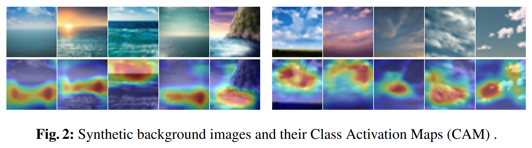
• To validate this phenomenon:
  • Generated synthetic images using Stable Diffusion:
    • One set with sea backgrounds only
    • Another set with sky backgrounds only
    • (No actual ships or airplanes included)
• Evaluation results (ResNet18 trained on CIFAR10):
  • 56.10% of sea images → classified as ship
  • 65.29% of sky images → classified as airplane
• CAM (Class Activation Map) analysis shows:
  • Model focuses on:
    • Sea horizon, waves
    • Clouds, sky patterns
  • → These are not intrinsic object features, but learned biases

3-3. Key Insight

• Even without target objects:
  • Models can classify inputs using bias-only information
• If a model had learned only object features:
  • It should randomly guess on such synthetic images
  • → But it does not

3-4. Motivation for Proposed Method

• Based on this observation:
  • Intentionally inject class-wise hidden biases into the dataset
• Expected outcome:
  • A model trained on such data will:
    • Learn both task features and embedded biases
• Key implication:
  • The model can classify bias-only inputs
  • → This property can be used to verify dataset usage

4. Method

• Bias has traditionally been regarded as a negative factor in deep learning because it can:
  • Degrade model performance
  • Introduce ethical problems such as gender or race bias
• For this reason, many previous studies have focused on debiasing techniques to remove such unwanted patterns
• In contrast, this paper takes a fundamentally different perspective:
  • It intentionally embeds class-wise hidden biases into the dataset
  • These hidden biases are used as a form of dataset watermark for copyright protection
• This main idea is:
  • Instead of eliminating bias, exploit it as a verifiable signal
  • A model trained on the watermarked dataset will learn these hidden class-specific biases
  • This learned behavior can later be used to verify whether the dataset was used during training

4-1. Noise Patch Placement: Class-wise Bias Embedding

• The first approach introduces class-specific noise patches into the dataset to embed hidden bias

4-1-1. Method

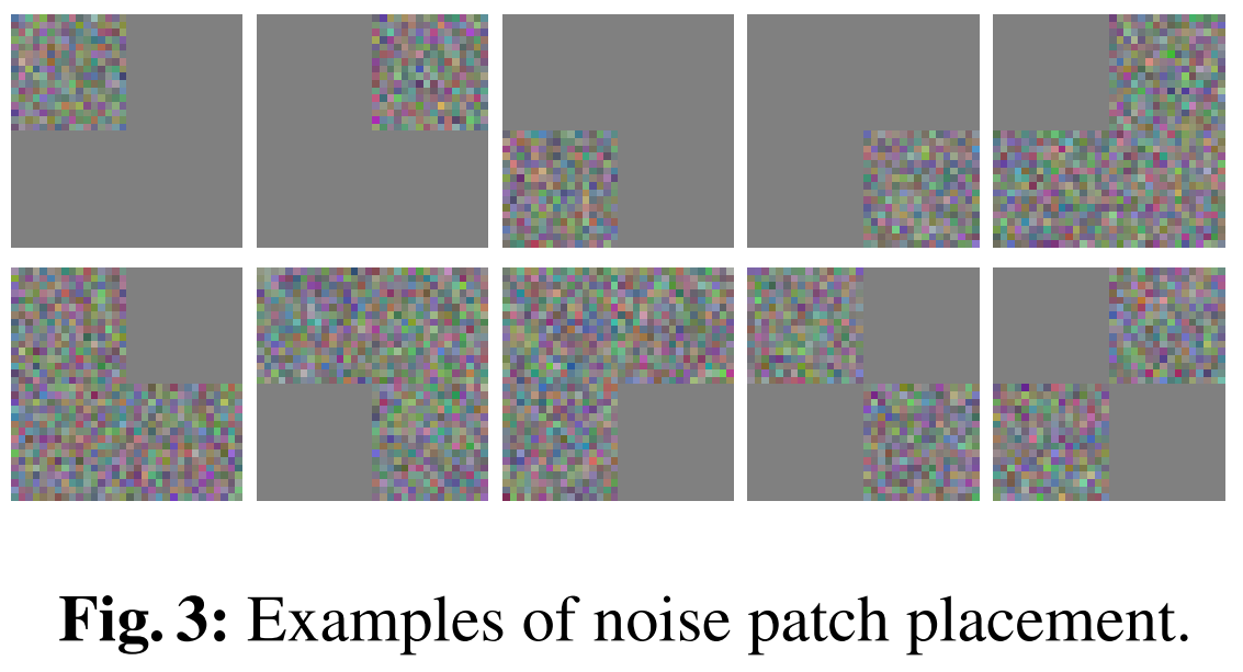
• For each class, a unique noise pattern is assigned and injected as:
  • $\hat{x} = x + \lambda n$ $s.t.$ $y^x = y^n$
    • $x$: original image
    • $n$: class-specific noise (Gaussian $\mathcal{N}(0,I)$)
    • $\lambda$: small scaling facotr (0.01)
    • Label remains unchanged (clean-labeled)
  • Note is:
    • Placed at predefined, class-specific spatial locations
    • Applied to 50% of training data

4-1-2. Experimental Setup

• Model: ResNet18
• Dataset: CIFAR10
• Training:
  • 100 epochs
  • Adam optimizer + cosine decay
  • Data augmentation applied
• Evaluation:
  • Tested on noise-only images

4-1-3. Key Findings

• Hidden bias can be embedded (clean-labeled)
  • Even though noise images are very different from original images:
    • Model achieves high accuracy on noise-only inputs
  • -> Confirms feasibility of watermark via noise placement
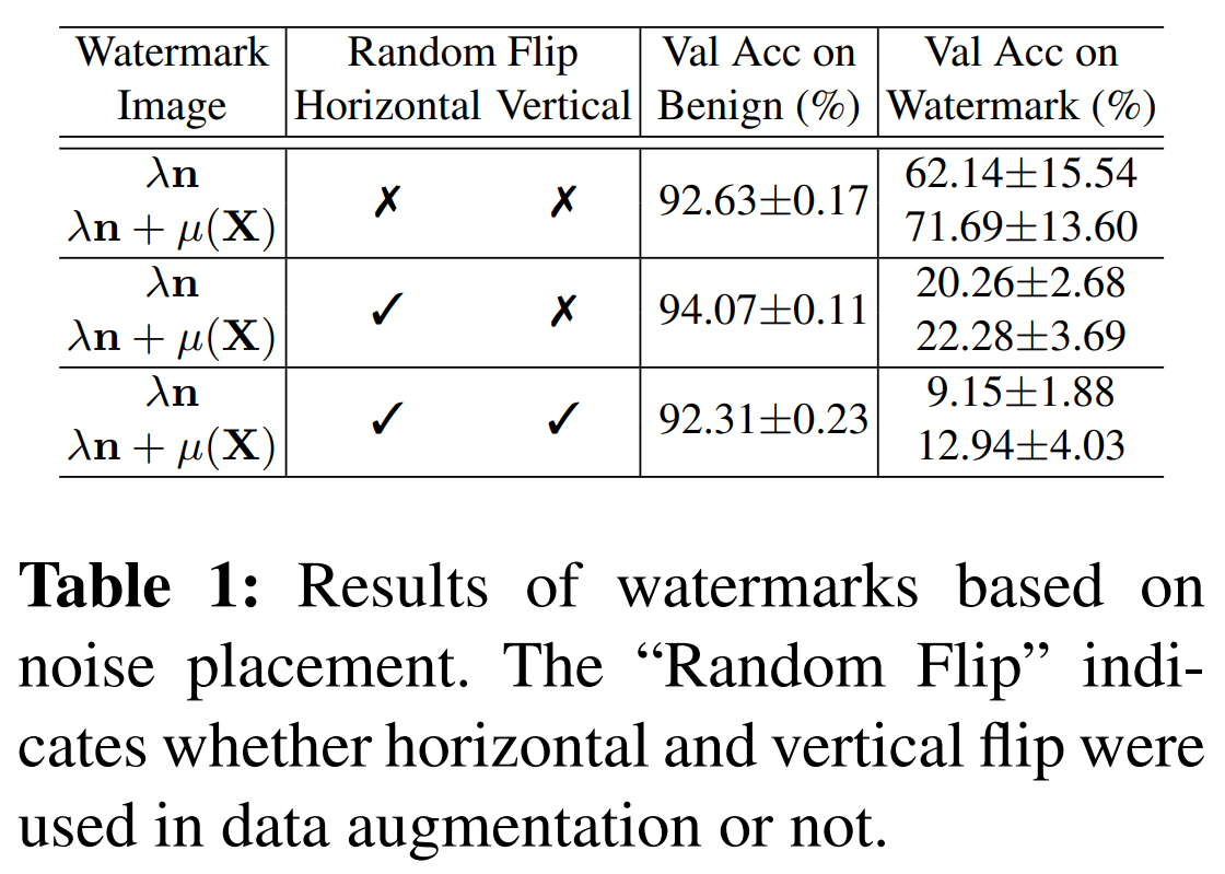
• Domain gap issue & solution
  • Performance:
    • $\lambda n$ alone -> lower accuracy
    • $\lambda n + \mu (\mathcal{X})$ -> higher accuracy
  • Reason:
    • $\lambda n$ has near-zero mean -> differs from real image distribution
    • Model tends to ignore it
  • Solution:
    • Add dataset mean $\mu (\mathcal{X})$
    • -> Aligns distribution -> improves classification
• Sensitivity to spatial transformations
  • Performance drops significantly with data augmentation:
    • No flip -> ~60% accuracy
    • Horizontal flip -> ~20%
    • Horizontal + vertical flip -> ~12%
  • Cause:
    • Noise patterns are location-dependent
    • Flip/rotations distort pattern consistency

4-1-4. Limitation

• Noise-based watermark is:
  • Not robust to spatial transformations (flip, rotation, translation)
• -> It leads to unstable verification

4-2. Overlaying Auxiliary Dataset: Robust Bias to Augmentation

• To address the lack of robustness to spatial transformations in noise-based methods, a more stable bias pattern is required

4-2-1. Method

• Instead of manually designing patterns, the method uses an auxiliary dataset to generate robust class-wise bias
• Watermarking is performed as:
  • $\hat{x}=(1-\lambda) x + \lambda x$ $s.t.$ $y^x=y^z$
    • $(z, y^z)$: auxiliary data and its label
    • $x$: target dataset sample
    • $z$: auxiliary dataset sample
    • $\lambda$: mixing coefficient
    • Labels are aligned (clean-labeled setting)

4-2-2. Label Alignment Strategy

• Even if two datasets are semantically unrelated:
  • Only class indices are matched
• Example:
  • select $x$ from CIFAR10: ‘airplane’ -> $y^x = $ ‘Class 0’
  • select $z$ from Fashion-MNIST: pullover -> $y^z = $ ‘Class 0’
  • -> corresponding $y^x$ and $y^z$ could both be denoted as ‘Class 0’
  • i.e., overlay both samples as same class

4-2-3. Experimental Setup

• Target dataset: CIFAR10
• Auxiliary dataset: Fashion-MNIST
• Model: ResNet18
• Training: same as noise patch experiment

4-2-4. Key Findings

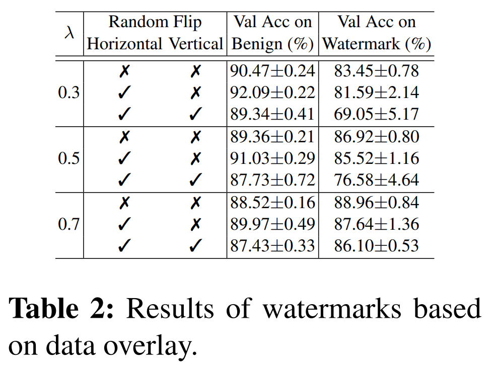
1. Strong robustness to augmentation
   • Overlaid patterns are:
     • Distributed across the image
     • Not tied to a specific location
   • -> Robust to flip, rotation, etc.
2. Effective hidden bias learning
   • Model successfully learns:
     • Auxiliary dataset patterns as class-specific bias
   • -> Works as a strong watermark signal

4-2-5. Limitations

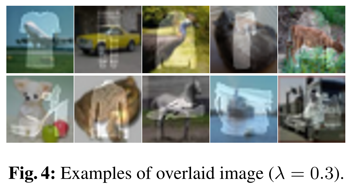
• Highly visible watermark
  • Overlay significantly alters image appearance
  • Easily detectable by human inspection
• Performance degradation
  • Large deviation from original data distribution
  • -> Lower validation accuracy on benign task
• Practical vulnerability
  • Can be removed or filtered visually

4-3. Undercover Bias: Invisible Bias Embedding

• Based on previous methods, an effective watermark must satisfy:
  1. Robustness to spatial transformations
  2. Near invisibility to human perception
• To achieve this, the paper proposes an invisible watermarking method using:
  • Image steganography
  • Auxiliary dataset

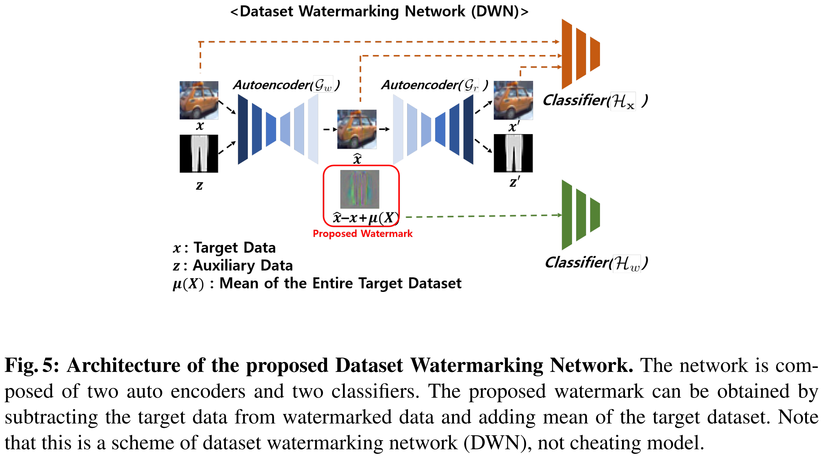
4-3-1. Overall Framework

• Watermarked image generation:
  • $\hat{x}=DWN(x,z)$
• Watermark definition
  • $w = \hat{x} - x$
  • $y^w = y^z$
    • $x$: original image
    • $z$: auxiliary image
    • $\hat{x}$: watermarked image
    • $w$: hidden watermark
    • Label of watermark follows auxiliary data

4-3-2. Dataset Watermarking Network (DWN)

• A neural network designed to:
  • Hide auxiliary information inside the image
  • While keeping the image visually unchanged
• Components
  1. Hiding Network ($G_w$)
     • Input: $x$, $z$
     • Output: $\hat{x}$ (visually similar to $x$)
  2. Reconstruction Network ($G_r$)
     • Input: $\hat{x}$
     • Output:
       • $x’$: reconstructed original image
       • $z’$: reconstructed auxiliary signal
         • $\hat{x}=G_w(x, z, \theta_{G_{w}})$
         • $x’,z’=G_r(\hat{x}, \theta_{G_{r}})$
       • $\theta_{G_{w}}$: weight of the autoencoder $G_w$
       • $\theta_{G_{r}}$: weight of the autoencoder $G_r$

4-3-3. Training Objective

• Train all components jointly using:
  • L1 loss (reconstruction)
  • Cross-entropy loss (classification)
• Loss components
  • Reconstruction constraints
    • Preserve original image: $\vert x - \hat{x} \vert$, $\vert x - x’ \vert$
    • Preserved embedded signal: $\vert z - z’ \vert$
  • Perceptual (classification) constraints
    • $H_x$: ensures original task performance
      • $x$, $\hat{x}$, $x’$ all classified correctly
    • $H_w$: ensures watermark encodes class-wise information
      • Extracted watermark corresponds to $y^z$
• Reconstruction loss
  • $\lambda_1^G \vert x - \hat{x} \vert + \lambda_2^G \vert x - x’ \vert + \lambda_3^G \vert z - z’ \vert$
    • $\vert x - \hat{x} \vert$: watermarked image should be close to the original (watermark invisibility)
    • $\vert x - x’ \vert$: reconstructed image $x’$ should match the original (prevent information loss)
    • $\vert z - z’ \vert$: embedded auxiliary information should be recoverable (ensures watermark is properly encoded)
• Origianl task loss (for classify $y^x$)
  • $\lambda_1^H \mathcal{L}{CE}(H_x(x), y^x) + \lambda_2^H \mathcal{L}{CE}(H_x(\hat{x}), y^x) + \lambda_3^H \mathcal{L}_{CE}(H_x(x’), y^x)$
    • $H_x(x)$: ensures correct classification of the original image (baseline)
    • $H_x(\hat{x})$: maintains performance even after watermark embedding (prevents degradation)
    • $H_x(x’)$: ensures reconstructed image is still meaningful and classifiable
• Watermark training loss (for classify $y^z$)
  • $\lambda_4^H \mathcal{L}_{CE}(H_w(x’ - x + \mu(X)), y^z)$
    • $x’ - x + \mu(X)$
    • $x’ - x = w$, i.e., watermark $w$
    • $\mu(X)$: mean image of the target dataset $X$
    • This formulation enables classification of auxiliary labels using only the watermark
• Final loss formulation
  • $\lambda_1^G \vert x - \hat{x} \vert + \lambda_2^G \vert x - x’ \vert + \lambda_3^G \vert z - z’ \vert + \lambda_1^H \mathcal{L}{CE}(H_x(x), y^x) + \lambda_2^H \mathcal{L}{CE}(H_x(\hat{x}), y^x) + \lambda_3^H \mathcal{L}{CE}(H_x(x’), y^x) + \lambda_4^H \mathcal{L}{CE}(H_w(x’ - x + \mu(X)), y^z)$

4-3-4. Practical Design Choice

• Instead of using many classifiers for model-agnostic training:
  • Use a simple CNN with dropout
  • Includes:
    • Spatial dropout
    • Standard dropout

4-3-5. Key Property

• After training:
  • Watermarked images can be generated without retraining
  • Watermarks are:
    • Invisible
    • Robust
    • Class-discriminative

4-4. Discussion

4-4-1. Issue: Number of Classes

• To ensure correct pairing:
  • $y^x = y^w$
  • -> Target data and watermark must share the same label
• Problem:
  • The auxiliary (watermark) dataset may have fewer or different number of classes than the target dataset
  • Direct one-to-one class matching becomes difficult
• Solution: Modulo Operation
  • $y^x \equiv y^w (mod N_{cls}^w)$
  • $N_{cls}^w$: number of classes in the watermark (auxiliary) dataset
  • Enables:
    • Flexible class pairing even when class counts differ
    • Reuse of watermark classes across multiple target classes

4-4-2. Verification Metric (Black-box Setting)

• Assumption:
  • Only predicted class outputs are available (strict black-box)
• Metric used: Mean Class Accuracy (mAcc)
  • $\frac{1}{N_{cls}^w} \sum_{c=1}^{N_{cls}^w} \mathbb{P}\big(F(\mu(X) + w, \theta_F) = c \mid y^w = k \big) > \tau$
• Key idea:
  • Evaluate model performance on watermark-only inputs:
    • $\mu(X) + w$
• Interpretation
  • Clean model
    • Has not seen watermark -> performs poorly (near random)
  • Cheating model
    • Learned watermark -> achieves high mAcc
  • Decision rule:
    • If mAcc $>$ threshold $\tau$ -> suspect dataset misues

4-4-3. Handling Different Class Sizes

• If target and auxiliary datasets differ in class count:
  • $F(\mu(X) + w, \theta_F) \equiv k (mod N_{cls}^w)$
• Ensures consistent evaluation under modulo mapping

4-4-4. Threshold Determination

• Goal:
  • Define a threshold that clean models cannot reach by chance
• Assumption
  • mAcc of a clean model follows:
    • Approximately Gaussian-like distribution
    • Centered at: {$\frac{1}{N_{cls}^w}$}

4-4-5. Trade-Off

• More precise thresholds:
  • Require estimating full distribution -> computationally expensive
• Proposed solution:
  • Use $2/N_{cls}^{w}$ as a lightweight and practical heuristic

5. Experiments I: Comparison with Prior Works

• This section compares the proposed method with:
  • Backdoor attacks
  • Data poisoning
  • Radioactive data
• Evaluation aspects:
  • computational cost
  • Invisibility
  • Harmlessness (impact on original task)
  • Verification ability
• Dataset used: CIFAR 10

5-0-1. Experimental Setup

• For all methods:
  • 50% of training data is watermarked/modified

5-0-2. Backdoor Attacks

• Two types considered:

1. Label-noised backdoor
   • Methods:
     • BadNets (Gu, et al., “Badnets: Evaluating backdooring attacks on deep neural networks”, IEEE Access 7, 2019.)
     • Blended (Chen, et al., “Targeted backdoor attacks on deep learning systems using data poisoning”, arXiv:1712.05526, 2017.)
   • Used only for basic specification comparison
2. Clean-labeled backdoor
   • Methods:
     • Hidden Trigger (Saha, et al., “Hidden trigger backdoor attacks”, AAAI, vol. 34, 2020.)
     • Sleeper Agent (Souri, et al., “Sleeper agent: Scalable hidden trigger backdoors for neural networks trained from scratch”, NeurIPS, 2022.)
   • Setup
     • 10 distinct triggers
     • One trigger assigned per class

5-0-3. Data Poisoning

• Methods:
  • Poison Frogs (Shafahi, et al., “Poison frogs! targeted clean-label poisoning attacks on neural networks”, NeurIPS, 2018.)
  • MetaPoison (Huang, et al., “Metapoison: Practical general purpose clean-label data poisoning”, NeurIPS, 2020.)
  • Bullseye (Aghakhani, et al., “Bullseye polytope: A scalable clean-label poisoning attack with improved tranferability”, EuroS&P, 2021.)
  • Gradient Matching (Geiping, et al., “Witches’ brew: Industrial scale data poisoning via gradient matching”. ICLR, 2021.)
• Setup:
  • 1 verification image per class
  • Total: 10 verification images
  • Multi-target setting
  • 5% poisoning budget per verification sample

5-0-4. Radioactive Data

• Method: Radioactive Data (Sablayrolles, et al., “Radioactive data: tracing through training”, ICML, 2020.)
• Setup:
  • 50% of training data marked
  • Entire test set also marked

5-0-5. Reference Model

• Required for prior methods:
  • Used ResNet18 trained on clean CIFAR10
• Implementation:
  • Below official codes were used
    • (Geiping, et al., “Witches’ brew: Industrial scale data poisoning via gradient matching”, ICLR, 2021.)
    • (Sablayrolles, et al., “Radioactive data: tracing through trainig”, ICML, 2020.)
    • (Souri, et al., “Sleeper agent: Scalable hidden trigger backdoors for neural networks trained from scratch”, NeurIPS, 2022.)

5-0-6. Proposed Method

• Approach
  • Embed watermark using auxiliary dataset (Fashion-MNIST)
• Architecture:
  • Pre-trained DWN (Dataset Watermarking Network)
    • Autoencoder: U-Net (Ronneberger, et al., “U-net: Convolutional networks for biomedical image segmentation”, MICCAI, 2015.)
    • Classifiers: Vanilla CNN (4 conv layers + dropout)
• Setup:
  • Watermark applied to 50% of training data

5-1. Comparison in Fundamental Specifications

5-1-1. Evaluation Criteria

• Harmlessness
  • Measured by validation accuracy on benign data
  • Higher accuracy -> less impact on original task
• Time Cost
  • Measured as watermarking time per image
  • Excludes:
    • DWN training time
    • Reference model training time
• Invisibility
  • Measured using SSIM (Structural Similarity Index)
  • Between:
    • Original image
    • Watermarked image

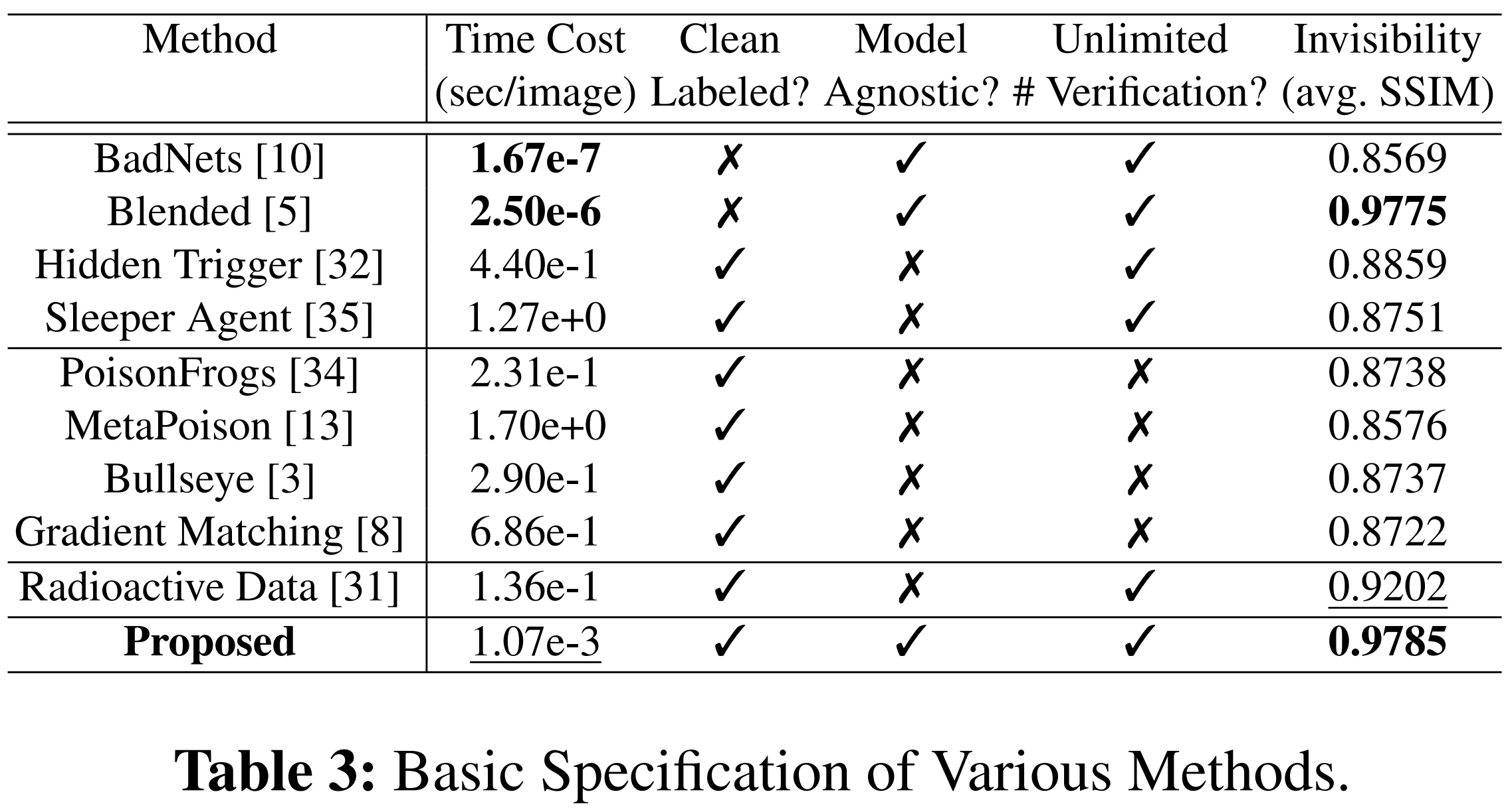
5-1-2. Observations on Prior Methods

• Label-noised backdoor attacks
  • Easily detectable via visual inspection
  • Due to incorrect labels
• Clean-labeled backdoor, data poisoning, radioactive data
  • Require reference models
  • -> Model-dependent
  • -> Computationally expensive
  • Often produce visible artifacts
• Data poisoning
  • Limited to a small number of victim samples
  • -> Weak scalability for verification

5-1-3. Advantages of Proposed Method

• High invisibility
  • Generate less perceptible watermarks
• Model-agnostic
  • Does not depend heavily on reference models
• Efficient
  • Faster watermarking process
• Scalable verification
  • No restriction on the number of watermark samples

5-2. Comparison in Effectiveness of Watermark

5-2-1. Purpose

• Evaluate effectiveness of watermarking methods in terms of:
  • Harmlessness (impact on original task)
  • Verifiability (ability to detect dataset usage)
• Compared methods
  • Backdoor attacks
  • Data poisoning
  • Radioactive data
  • Proposed method

5-2-2. Experimental Setting

• Dataset: CIFAR10
• For all methods:
  • 50% of training data randomly watermarked

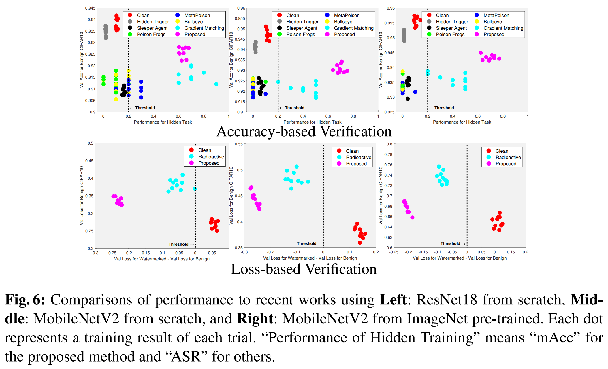
5-2-3. Training Scenarios

• Experiments conducted under three settings
  1. ResNet18 (from scratch)
  • 100 epochs
    1. MobileNetV2 (from scratch)
  • 300 epochs
    1. MobileNetV2 (ImageNet pre-trained)
  • 100 epochs
• Each scenario:
  • Repeated 10 times
  • With data augmentation

5-2-4. Evaluation Metrics

1. Harmlessness
   • Measured using validation accuracy on benign dataset
   • For data poisoning, excluded 10 verification images to ensure fair evaluation
2. Verification Ability
   • Backdoor attacks & Data poisoning
     • ASR (Attack Success Rate)
       • Measures success rate of intended misclassification
   • Radioactive data
     • Difference between:
       • Validation loss on benign data
       • Validation loss on radioactive-marked data
   • Proposed method
     • Uses multiple metrics:
       • mAcc (mean class accuracy on watermark)
       • ASR
       • Loss difference

5-3. Results

6. Experiments II: General Applicability

• The previous experiments validated the method in limited settings (mainly CIFAR10)
• This section evaluates whether the proposed method:
  • Generalizes across datasets
  • Works on different model architectures
  • Remains effective under varied tasks

6-1. Application to Further Architectures and Datasets

6-1-1. Purpose

• Extend evaluation beyond CIFAR10 and a few models
• Verify robustness and general applicability of the method

6-1-2. Experimental Setting

• Datasets
  • CIFAR100 (100 classes)
  • FER2013 (7 classes)
  • Fashion-MNIST
• Compared Methods
  • Backdoor attack: Sleeper Agent (best-performing prior method)
  • Data poisoning: Gradient Matching (best-performing prior method)
• Models
  • Reference models
    • ResNet18
    • Simple (benign) CNN
  • Cheating models
    • DenseNet-BC (trained from scratch)
• Auxiliary Datasets
  • CIFAR100: Fashion-MNIST + MNIST (each with 10 classes)
  • FER2013: First 7 classes of MNIST
• Additional Architecture Evaluation
  • Test on CIFAR10 (target) + Fashion-MNIST (auxiliary) with:
    • EfficientNet
    • PVTv2
    • ResMLP
    • PiT
  • Training Setup:
    • ImageNet pre-trained initialization
    • 35 epochs
    • SGD optimizer
    • Warmup + label smoothing
    • Data augmentation: Spatial transformations, Mixup
    • Multiple runs for robustness

6-1-3. Results

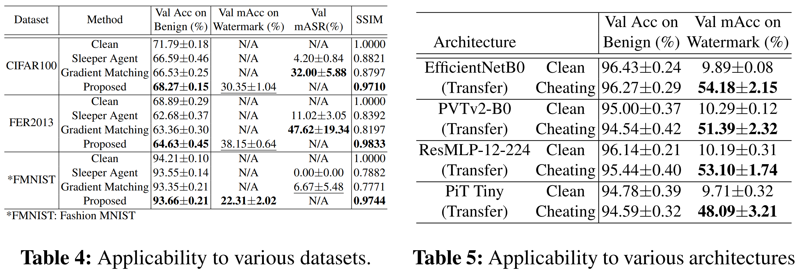
• The proposed method consistently demonstrates
  1. Harmlessness: Minimal degradation in original task performance
  2. Invisibility: Watermarks remain imperceptible across datasets
  3. Verifiability: Strong performance in detecting dataset usage

6-1-4. Additional Findings

• mAcc (watermark classification accuracy):
  • Consistently higher than prior methods across architectures
• Threshold performance:
  • Achieved 100% accuracy in distinguishing:
    • Clean models vs. cheating models

6-2. Application to Fine-grained Classification

6-2-1. Purpose

• Address a key limitation:
  • Auxiliary dataset is typically required to have equal or more classes than the target dataset
• Solution:
  • Use modulo operation to enable class matching even when target dataset has more classes than auxiliary dataset

6-2-2. Experimental Setting

• Datasets
  • Tiny ImageNet (100 classes)
  • ImageNet (1,000 classes)
  • Auxiliary dataset:
    • Fashion-MNIST (10 classes)
• Setup
  • 50% of training data watermarked
  • Model: MobileNetV2
  • Training configurations:
    1. Tiny ImageNet
       • Trained from scratch
       • SSIM: 0.9883
    2. ImageNet
       • Initialized from pre-trained ImageNet model
       • SSIM: 0.9570

6-2-3. Results

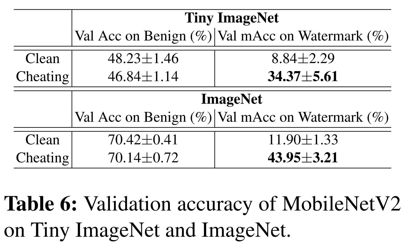
• Based on multiple trials:
  • Tiny ImageNet: 30 runs
  • ImageNet: 5 runs
• Harmlessness: Slight decrease in validation accuracy on benign data
• Verifiability: Significant improvement in detecting watermark signals
• Clean model behavior: Performance on watermark inputs drops to near chance level

6-2-5. Implication

• Even when target dataset has far more classes than auxiliary dataset -> The proposed method still works effectively

6-3. Application to Image Segmentation

6-3-1. Purpose

• Extend the proposed watermarking method from image classification to image segmentation
• Key challenge:
  • Segmentation requires pixel-level predictions, not image-level labels

6-3-2. Method Adaptation

• Introduce spatially varying watermarks:
  • Auxiliary data is:
    • Resized to small patches (e.g., 8x8 pixels)
    • Repeatedly stitched onto image segments
  • Each patch is aligned with:
    • The label of the corresponding segment
• Applied to 50% of PASCAL VOC 2012 dataset

6-3-3. Model Adjustment

• Modified DWN:
  • Replace classification heads with autoencoders + dropout
• Backbone:
  • MobileNetV2
• Training setup:
  • From scratch
  • Adam optimizer (initial LR = 1e-3, with decay)
  • Batch size = 60
  • Data augmentation applied

6-3-4. Threshold Adjustment

• In segmentation:
  • Important information lies in object shapes (silhouettes)
• Therefore:
  • Requires a higher verification threshold than $\frac{2}{N_{cls}^w}$

6-3-5. Evaluation Metrics

• Task performance
  • Measured by mIoU (mean Intersection over Union)
• Verification
  • Measured by:
    • Mean class pixel accuracy
    • On masked (watermark) regions

6-3-6. Results

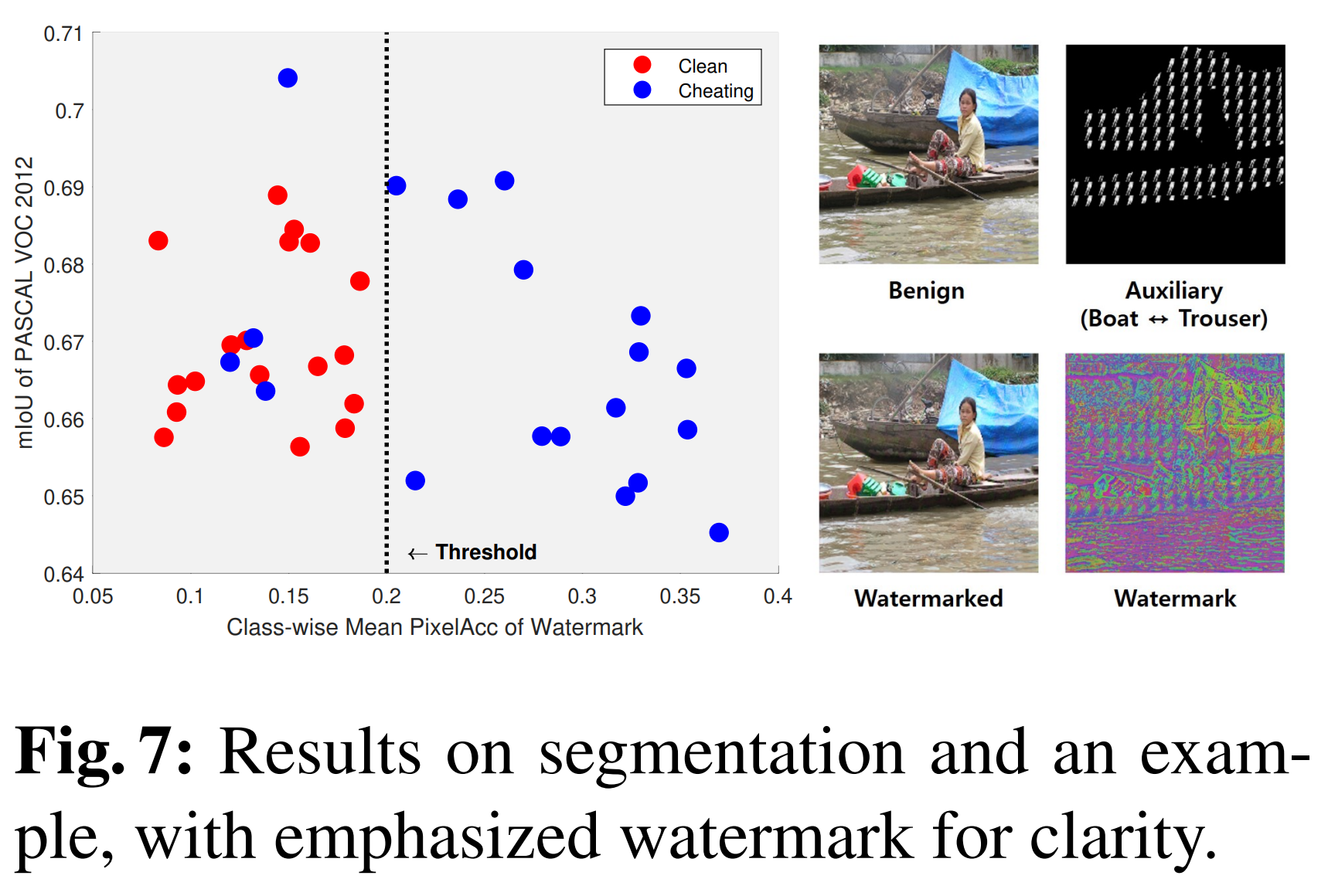
• Harmlessness
  • Minimal degradation in segmentation performance
• Verifiability
  • Watermark successfully learned in most trials
• Performance comparison
  • Clean models: accuracy < 0.2
  • Cheating models: 79% of trials -> accuracy > 0.2

7. Ablation Studies

7-1. Histogram Analysis of mAcc on Watermark

7-1-1. Purpose

• Validate the threshold criterion used for detecting cheating models
• $\tau = \frac{2}{N_{cls}^w}$

7-1-2. Experimental Setting

• Models:
  • ResNet18 on CIFAR10
  • DenseNet on CIFAR100
• Training:
  • With and without watermark
  • From scratch
  • Optimizer: Adam (learning rate = 1e-3)
  • Epochs: 100
• Scale:
  • 300+ training runs per setting
• Evaluation:
  • Measure mAcc on watermark
  • Analyze distribution via histograms

7-1-3. Results

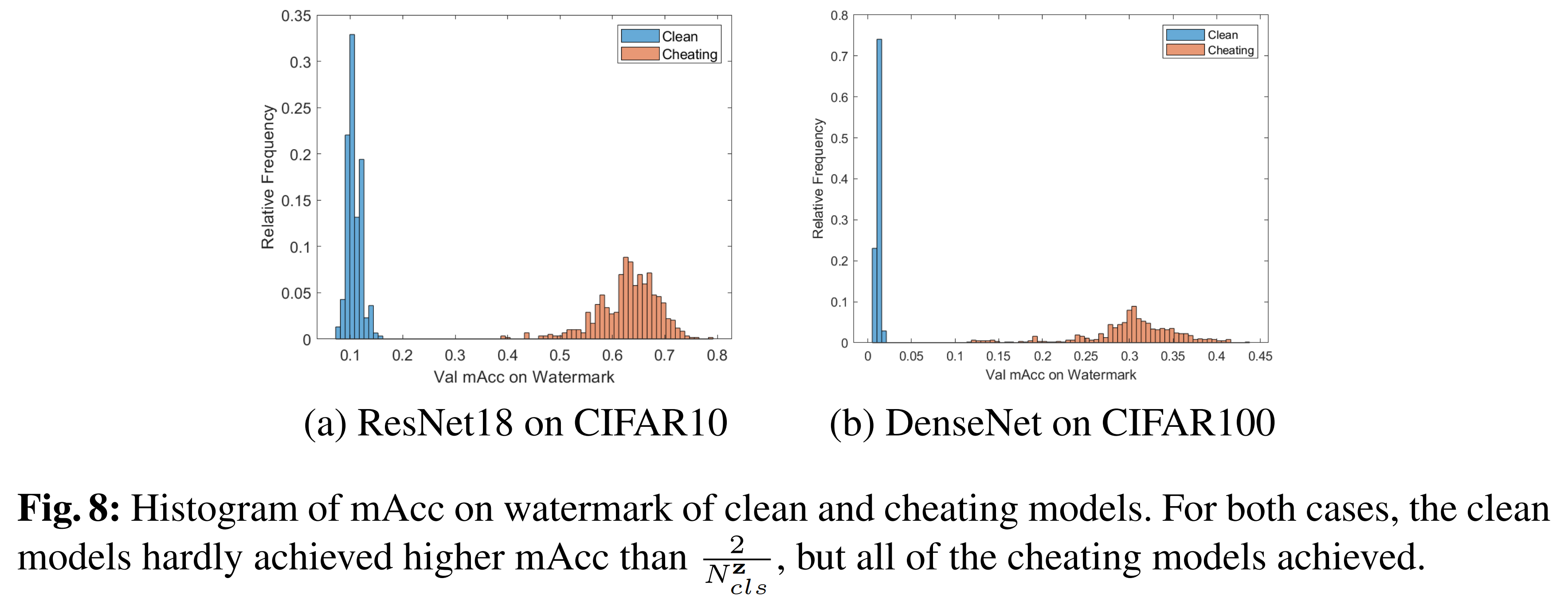
• mAcc values follow a Gaussian-like distribution

• Observations

  • Clean models rarely approach to $\frac{2}{N_{cls}^w}$
  • Chaeting models all exceed $\frac{2}{N_{cls}^w}$
  • No samples observed:
    • At 0% mAcc
    • At exactly $\frac{2}{N_{cls}^w}$

7-1-4. Statistical Interpretation

• Threshold: $\frac{2}{N_{cls}^w}$
• Corresponds to: ~7× and ~5× standard deviation from the mean
• Clean model exceeding threshold probability: $< 3 \times 10^{-5}$

7-2. Visualizations

7-2-1. Purpose

• Analyze how the watermark is learned using:
  • t-SNE (feature space visualization)
  • CAM (Class Activation Map)
• Goal:
  • Understand whether models actually learn hidden bias (watermark)

7-2-2. Experimental Setting

• Two models trained:
  • Clean model: trained on benign CIFAR10
  • Cheating model: trained on watermarked CIFAR10
• Procedure:
  • Extract last-layer latent features
  • Visualize using:
    • 2D t-SNE plots
    • CAM heatmaps

7-2-3. Results

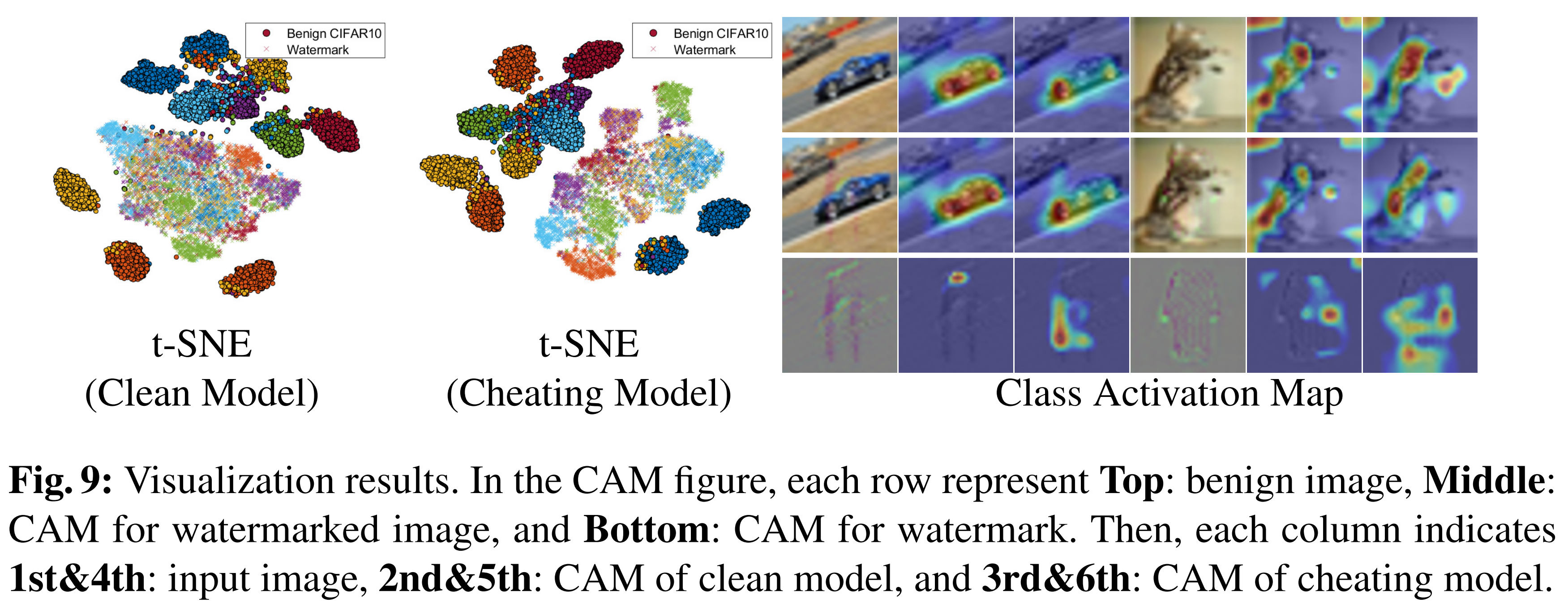
• t-SNE Analysis
  • Benign data
    • Both clean and cheating models show clear and well-separated clusters
    • -> Normal feature learning
  • Watermark data
    • Cheating model shows partial clustering
    • Clean model shows no clustering structure
  • Interpretation: Only the cheating model learns meaningful representations of watermark
• CAM Analysis
  • Cheating model
    • Responds to benign images, watermarked images, watermark-only inputs
  • Clean model
    • Responds only to benign images
    • Ignores watermark signals

8. Conclusion & Limitations

• This paper proposes “undercover bias”, a novel dataset watermarking method:
  • Embeds class-wise hidden bias into the dataset
  • Enables detection of models trained on that dataset

8-1. Core Idea

• Models trained on watermarked data:
  • Unintentionally learn hidden bias
  • Respond to watermark signals
• This behavior serves as evidence of dataset misuse (cheating)

8-2. Key Contributions

• Observed that:
  • Models can classify background-only images
  • → Indicates unintended bias learning
• Developed two preliminary methods:
  • Noise patch placement
  • Dataset overlay
• Identified key requirements:
  • Robustness to spatial transformations
  • Invisibility
• Proposed final method:
  • Undercover bias satisfying both requirements

8-3. Effectiveness

• Compared to prior methods:
  • More reliable verification
  • Less visible watermark
  • Less impact on task performance
• Additional validation:
  • Ablation studies
  • Visualization analysis

8-4. Generalization

• Successfully applied to:
  • Fine-grained classification
  • Image segmentation
• Demonstrates:
  • Broad applicability across tasks and settings

8-5. Limitations

• Not applicable to text data
  • Small perturbations can drastically change meaning
• Slight performance degradation
  • Watermarked models perform marginally worse than clean models